About cms package
In our paper “Design of composite measure schemes for comparative severity assessment in animal-basedneuroscience research: a case study focussed on rat epilepsy models” (Dijk et al. 2020), we introduce composite measures schemes (cms) to assess severity in rat epilepsy models. We suggest a PCA-based algorithm to assess a plethora of outcome variables for their suitability as features in a simple composite score for comparative severity assessment.
This vignette covers the basic functions for cms analysis in R (R Core Team 2019).
Package Requirements
In order to use the cms package, some dependencies need to be installed. Please make sure to install the following R-packges from CRAN before using cms.
ggplot2 (Wickham 2016)
dplyr (Wickham et al. 2021) factoextra (Kassambara and Mundt 2020)
install.packages("ggplot2")
install.packages("dplyr")
install.packages("factoextra")
Code and information
For more information on the cms package and the source code see:
- cms website and
- the cms GitHub repository
Introduction
According to the EU directive 2010/63 it is essential to assess the severity of interventions and models in experimental animals. Therefore, sensitive and robust parameters are crucial. Based on the data generated in three different epilepsy models, promising parameters were selected and combined to a composite measure scheme. The cms package guides through the process of selecting potential parameters or to allocate your animals to clusters based on the cms. Related to the pre-defined or individual selection and combination of parameters, the respective clusters and the distribution of the animals to these clusters will be visualized.
The calculated clusters describe different levels of severity. Please consider that the “best” parameters can vary in different models, species or even between different laboratories. Therefore, this tool can help selecting the most interesting parameters from individually generated data.
For the interpretation of the different severity levels, one has to consider that they are based on the highest severity animals experienced in the experiments but not necessarily the highest existing. Moreover, there might always be “better” parameters. So be aware of the limitations of the individually created cms.
In conclusion, the cms package is a useful tool to get a retrospective overview of the severity in animal data experienced during an xperiment. Therefore, it can help to complement a mostly empiric severity assessment.
What the cms package…
| … can do | … can’t do |
|---|---|
| Helps to select interesting parameters for severity assessment | Interpretation of the selected parameters in terms of how useful they can be to assess the impairment of animals’ wellbeing |
| Provides a basis for quantitative and comparative severity assessment (incl. comparison with data from the different epilepsy models) | |
| Allocation of individual animals to a severity level | Direct translation of the different severity levels to those of the EU directive 2010/63 |
| Be a useful tool to complement an empiric severity assessment in an objective and scientific way | Replace the common severity assessment |
Data structure
The cms algorithm requires the input data in specific long format. The table can be combined with meta information. The user has to specify a column from which on only measurement data are included. Before that column all entries can have informative character.
Meta-information (=column headers) in the included data are:
- shortname a short term study identifier (e.g., kindling)
-
for2591_id internal identifier
- species analysed species
- sex analysed sex
- strain animal strain id
- animal_id animal identifier (mandatory!)
- treatment experimental treatment (mandatory!)
- subproject subproject (mandatory if there are subprojects!)
- groups subgroups (mandatory if there are additional subgroups in the data)
- mod model string (e.g., chem, elec, kind)
- repeats experimental repeats (mandatory!); if only one repeat set this column to 3
Please note that most of the presented meta-data are optional. However, you may use any of the included criteria to filter the datafor subsets.
Measurement data in the provided example start at column No. 14. The following 57 variables are included. Note that the raw data include a lot of missing values (NA). These can be curated in the algorithm using the emptysize object.
Bwc, rgs, tint_mouse, nesting_rat, burrowing_rat, openfield_rat, cort_plasma, cort_fec, cort_fur_hair, food, social_interaction, Sacc_pref, OF_rearing_frequency, Of_immobile_duration, OF_center_time, BWB_WB, BWB_entries_in_BB, BWB_streching, BWB_LT, EPM_stretching, EPM_head_dip, EPM_closed_arms_duration, EPM_open_arms_duration, EPM_open1_3, Adrenal_glands, Creatincinase, Oxytocin, BDNF, Irwin, Seizures_n, Seizures_duration, Act_d, Act_n, HR_d, HR_n, NN.I_d, NN.I_n, NNx_d, NNx_n, pNNx_d, pNNx_n, RMSSD_d, RMSSD_n, SDNN_d, SDNN_n, MPPF_hippocampus_L, MPPF_hippocampus_R, MPPF_mPFC, MPPF_septum, FDG_mPFC, FDG_septum, FDG_amygdala, FDG_striatum, FDG_hypothalamus, FDG_thalamus, FDG_parietal_cortex, FDG_hippocampus
The full data are included in the cms package and can be accessed with:
library(cms)
head(episet_full)
Minimum data
The cms function requires a minimum on information to work. Depending on the number of subsets, the mandatory table fields are:
animal_id
treatment (e.g., “naive”, “sham” and “SE”)
mod (e.g., “chem”, “elec” and “kind”)
variables (e.g., burrowing, corticosterone, openfield,…)
The treatment and mod columns can be used for subsetting or pooling the data.
Example 1
Let’s analyze repeat No. 3 from the episet_full and use the a battery of 23 variables in the data to extract features. Note, that this analysis uses the pooled treatment (“naive”, “SE” and “sham”) and mod (“chem”, “elec” and “kind”) argument.
# first we select only the repeats = 3
set       <- cms::episet_full[episet_full$repeats %in% 3, ]

# Now the variables that shall be testes are called in a vector
variables <- c("Sacc_pref", "social_interaction",
               "burrowing_rat", "openfield_rat")

# do the cms feature analysis
features  <- cms(raw        = set,
                 runs       = 300,
                 idvariable = "animal_id",
                 setsize    = 0.8,
                 variables  = variables,
                 maxPC      = 1:3,
                 clusters   = 3,
                 showplot   = FALSE,
                 legendpos  = "none")
features$p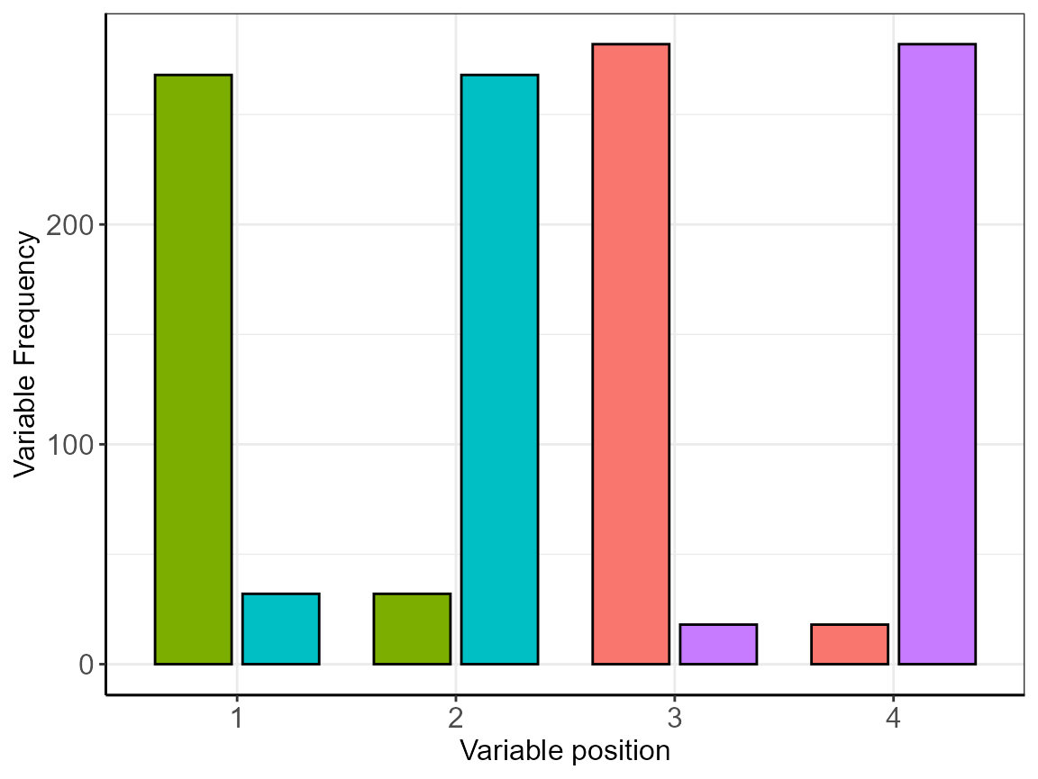
Feature distributions after cms analysis.
The plot is rather crowded so that the information we are seeking is better extracted from the attached frequency (features$FRQ) table. Only looking at the first 10 rows.
| position | x | freq | perc |
|---|---|---|---|
| 1 | openfield_rat | 268 | 89.33 |
| 1 | Sacc_pref | 32 | 10.67 |
| 2 | openfield_rat | 32 | 10.67 |
| 2 | Sacc_pref | 268 | 89.33 |
| 3 | burrowing_rat | 282 | 94.00 |
| 3 | social_interaction | 18 | 6.00 |
| 4 | burrowing_rat | 18 | 6.00 |
| 4 | social_interaction | 282 | 94.00 |
The result shows the following feature order in repeats=3, with the above listed variables, using 4 principle components in 100 repeated runs: BWB_WB (40%) > BWB_LT (32%) > Adrenal_glands (20%) > cort_fec (6%) > openfield_rat (1%) > social_interaction (1%).
The remaining variables were not selected and/or not contributing to the PCA. Therefore, they were not deemed to be relevant features.
Cluster analysis
The cms function also calculates a composite score from the principal component scores. This “compscore” is simply the sum of the 1 to maxPC PCA scores. The result is stored in the result of the cms function as a list object. In the upper example, we can access this information with features$reportdata$compscore.
The observant reader might have noticed the clusters=3 object in the cms function. This is the number of clusters that shall be applied to the “compscore”. Unfortunately, this is a heuristic. This means: the user will have to figure out how many clusters are correct for the data. The cluster information, or better: the distribution of the clusters are characteristic for specific subgroups.
Fortunately, the cms function takes care of the heuristic determination of the number of clusters. The weighted sums of squares are calculated with the 1 to maxPC PCA scores of the data and the selected number of clusters is marked with a vertical line. With the Kaiser-Guttman criterion (“ellbow method”) the ideal number of clusters can be inferred.
features$pscree
#> NULL
Now it becomes clear, why we have kept the subgroup information in the feature extraction above. We can easily control the subgroups with the dplyr package and plot the cluster distributions. The plot_cms function will take care of this.
cms_clustering <- plot_cms(cmsresult = features,
                           rotateX   = 45)
cms_clustering$p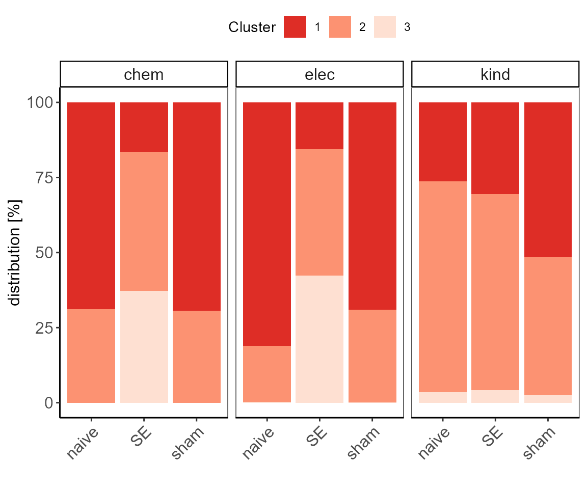
Cluster frequencies after cms analysis.
| treatment | mod | cluster | n | freq |
|---|---|---|---|---|
| naive | chem | 1 | 3955 | 68.8664461 |
| naive | chem | 2 | 1788 | 31.1335539 |
| naive | elec | 1 | 4462 | 81.1272727 |
| naive | elec | 2 | 1026 | 18.6545455 |
| naive | elec | 3 | 12 | 0.2181818 |
| naive | kind | 1 | 760 | 26.3249047 |
| naive | kind | 2 | 2027 | 70.2112920 |
| naive | kind | 3 | 100 | 3.4638033 |
| SE | chem | 1 | 1545 | 16.5399850 |
| SE | chem | 2 | 4330 | 46.3547800 |
| SE | chem | 3 | 3466 | 37.1052350 |
| SE | elec | 1 | 967 | 15.6776913 |
| SE | elec | 2 | 2596 | 42.0881971 |
| SE | elec | 3 | 2605 | 42.2341115 |
| SE | kind | 1 | 890 | 30.6685045 |
| SE | kind | 2 | 1892 | 65.1964163 |
| SE | kind | 3 | 120 | 4.1350793 |
| sham | chem | 1 | 4990 | 69.4599109 |
| sham | chem | 2 | 2194 | 30.5400891 |
| sham | elec | 1 | 4152 | 69.0963555 |
| sham | elec | 2 | 1854 | 30.8537194 |
| sham | elec | 3 | 3 | 0.0499251 |
| sham | kind | 1 | 1478 | 51.5701326 |
| sham | kind | 2 | 1313 | 45.8129798 |
| sham | kind | 3 | 75 | 2.6168876 |
References
Dijk, Roelof Maarten van, Ines Koska, Andre Bleich, Rene Tolba, Isabel Seiffert, Christina Möller, Valentina Di Liberto, Steven Roger Talbot, and Heidrun Potschka. 2020. “Design of Composite Measure Schemes for Comparative Severity Assessment in Animal-Based Neuroscience Research: A Case Study Focussed on Rat Epilepsy Models.” PLOS ONE 15 (5): 1–17. https://doi.org/10.1371/journal.pone.0230141.
Kassambara, Alboukadel, and Fabian Mundt. 2020. Factoextra: Extract and Visualize the Results of Multivariate Data Analyses. https://CRAN.R-project.org/package=factoextra.
R Core Team. 2019. R: A Language and Environment for Statistical Computing. Vienna, Austria: R Foundation for Statistical Computing. https://www.R-project.org/.
Wickham, Hadley. 2016. Ggplot2: Elegant Graphics for Data Analysis. Springer-Verlag New York. https://ggplot2.tidyverse.org.
Wickham, Hadley, Romain François, Lionel Henry, and Kirill Müller. 2021. Dplyr: A Grammar of Data Manipulation. https://CRAN.R-project.org/package=dplyr.