RELSA Score

RELSA: Relative Severity Assessment (RELSA) Score

The relsa function from the RELSA package allows the calculation of a (composite) score for relative severity assessment in individual animals using collections of experimental outcome variables or single parameters. The RELSA Vignette covers how to load, access, and calculate RELSA scores in detail.

This Vignette aims to provide a better understanding of what RELSA is, how it is calculated, and what it can be used for.

RELSA scores express severity in two ways:

The score provides a metric for direct comparison within a relative context.
Relative context is established by providing a reference model with assumed (biological) severity.

There is a possible third option in which k-means clustering is applied to the baseline model to obtain k-levels within the data range. This way, an unbiased subsetting of the calculated scores into classes is achieved (for further classification analysis, etc.).

Thus, animals from different experimental backgrounds and conditions can be compared. However, it is essential to note that the RELSA score reflects what happens in the measured data. If the data, for some reason, do not reflect severity in animals, the RELSA score might be unsuited for comparisons.

RELSA calculation

This section explains how the RELSA score is calculated step by step. The relsa function accepts normalized data in the RELSA format. How these tables are built is explained in detail in the RELSA Vignette.

The function requires a reference model for establishing a relative context within an animal model with “known” severity. This severity can be qualitative as tested animals will always be compared to this model - thus, the word “relative” in RELSA. The drop object variables can be excluded from the current analysis. turnvars defines variables where measured values increase rather than decrease when severity impacts the animal.

# RELSA function
relsa (set, bsl, a=1, drop=NULL, turnvars=NULL)

Subsetting of the normalized test data

The resulting table of normalized variables looks like the following example for a transmitter-operated mouse with six outcome measures. Sometimes, not all of them are needed in the RELSA calculation. For example, variables can be dropped with the drop object.

(bw, bwc and clinical score are strongly correlated so that just bwc is used; further, mouse grimace scale 30 min and 180 lack baseline values and show missing data on the following days, so they will be skipped here as well).

day	bwc	burON	hr	hrv	temp	act
-1	100.00	100.00	100.00	100.00	100.00	100.00
0	87.50	62.12	145.65	16.50	98.83	11.79
1	90.76	135.72	128.96	38.96	102.42	38.25
2	92.93	137.62	118.63	54.44	101.44	33.02
3	94.02	NA	106.30	56.89	100.27	26.88
4	94.02	96.13	115.87	57.39	101.29	36.37

Calculation of differences

In the next step, differences to baseline values are calculated. As the baseline is 100 % in both “directions” (increasing and decreasing values), the approach is rather straight forward:

for decreasing values
delta = 100 - subdata[-1]
for increasing values
delta = 100 - subdata[-1]
delta[,turnvars] = delta[, turnvars]* -1

With [-1] the daily baseline values at day=-1 are not recognized in the calculation.

Also - after this step - all differences <0 are set to 0 so that there are no negative values. A negative value indicates a full recovery. Negative values play no role in the RELSA calculation so that they are eliminated. Zeros also point to non-missing but recovered data. This difference is essential since missing values will not contribute to mathematical calculations such as the mean. This would skew the results and give weight to variables not present in the data.

An example for a cleaned difference matrix (D) is shown in the following example (in which the no variables were dropped and two turned: c(“hr”, “temp” ). Missing data are indicated as NAs.

#> NULL

bwc	burON	hr	hrv	temp	act
0.00	0.00	0.00	0.00	0.00	0.00
12.50	37.88	45.65	83.50	0.00	88.21
9.24	0.00	28.96	61.04	2.42	61.75
7.07	0.00	18.63	45.56	1.44	66.98
5.98	NA	6.30	43.11	0.27	73.12
5.98	3.87	15.87	42.61	1.29	63.63

Calculation of the RELSA score

The baseline model is required for context. The values in the baseline model show the extrema for each variable in the current model. They are the maximum (or minimum) reached values coding for some virtually known or prospective severity. Every test animal with its unique values and variables will be compared to these baseline values arithmetically to yield a RELSA weight factor (RW), which is also an effect size - regularized to the maximum deviation of the reference set.

\[RW=\frac{|100-i|}{|100-max_i,ref)|}\] For example, if the lowest reached body weight change (bwc) value in an animal of the training data is, e.g., 15 % and the actual loss in a test animal is 11 %, RW results to RW=(100-89)/(100-85) = 0.73. In other words, the actual mouse reached 73 % of the maximum bwc deviation of the baseline data. Since context is relevant here, this also means that the animal also experiences 73 % of the utmost reached severity of the baseline model. This is repeated for each day and available variable.

Following the example above, the resulting RELSA weights (RW) are represented in the following matrix:

bwc	burON	hr	hrv	temp	act
0.00	0.00	0.00	0.00	0.00	0.00
0.81	0.38	0.85	0.91	0.00	0.92
0.60	0.00	0.54	0.66	0.55	0.65
0.46	0.00	0.35	0.50	0.33	0.70
0.39	NA	0.12	0.47	0.06	0.76
0.39	0.04	0.30	0.46	0.29	0.67

The weights show the magnitude of variable deviation. They generalize the mean differences in each animal that are further regularized by the extrema of the reference model. Calculating the mean for these values will not reflect the actual situation in terms of severity because we are looking for the extrema indicating potential severity, magnitude matters. In statistics, this is traditionally solved by squaring numbers. Therefore, we deem the combined weight factor’s root mean square (RMS) as a reasonable choice for the final RELSA score calculation - giving larger deltas (weights or effects) more weight.

\[RELSA(t)=\sqrt{\frac{1}{n}\sum_{i=1}^n (RW)_i^2}\]

day	RELSA
-1	0.00
0	0.73
1	0.55
2	0.44
3	0.44
4	0.41

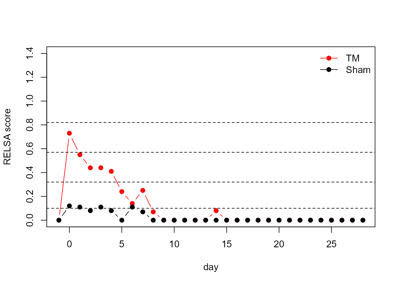
Use-case: Comparison of sham vs. transmitter-implanted mice

In the end, comparisons between, e.g., sham and transmitter-operated animals are possible. In the following example, seven six variables are used to calculate the respective RELSA scores (time points are days here). Day=-1 is the baseline physiological state, and day=0 is a post-operational state with the expected maximum severity.

It can be seen that the relative severity of the transmitter implantation is more prominent than in the sham-operated animal. However, the course of both lines is somewhat similar, indicating that experimental procedures are very well reflected in each of the two cases, and differences can be attributed to differences in severity.