simsalRbim Examples

Preference Tests

For this vignette, we will use the artificial dataset “ZickeZacke”, a perfectly balanced set of paired-choices preference tests, integrated in simsalRbim. In this dataset, every subject was tested with every possible item combination, but one item (“HoiHoiHoi”) was tested with only 3 subjects (eins, zwei & vier).

In addition, there is one item combination with “HoiHoiHoi” that resulted in equal responses (no preference, ties: subjectID=vier, HoiHoiHoi vs Kacke). Thus, we have a ground truth dataset whereof we know the ranking (“Zicke” > “Zacke” > “Huehner”> “Kacke”) and one item that we do not know the exact position within that ranking. Let’s see if we can evaluate the item’s position by employing three different strategies which are covered by the following examples.

Example 1 - The calculation of worth values

First, the data are loaded. In this example, internal data are used. You can use the bimload function to import data from a variety of formats.

Define the item to be tested (simOpt) and a Ground Truth (GT) of items that it is tested with. Any items that are not defined here, will not be used in the analysis. This may lead to incomplete conclusions. So be careful with what you put in here. The simOpt and GT objects are then used in the bimpre function to preprocess the data into a unified format and bimpre also identifies ties. As you can see from the example below, the ties get marked in the ‘tie’ column.

dat        <- ZickeZacke

simOpt     <- "HoiHoiHoi"
GT         <- c("Zicke", "Zacke", "Huehner", "Kacke" )

predat     <- bimpre(dat=dat, GT=GT, simOpt=simOpt)
#> simsalRbim: 1 tie(s) marked.

In the next step, we calculate the worth values of all items specified in the simOpt and the GT term. This uses a non-linear GNM model from the prefmod[1] package to model the data and to transform the estimates into worth values. The showPlot object can be set to “worth” providing the worth values, or “coef” providing the model coefficients in the output.

Note, that if randOP is set to TRUE, the attribution of ties in terms of the dependent results variable in the GNM model will be random. This means that each time this function is executed, the worth values will change. This is an integral part of this package and will be used in the simulations later.

worth      <- bimworth(ydata    = predat,
                       GT       = GT,
                       simOpt   = simOpt,
                       randOP   = FALSE,
                       showPlot = "worth",
                       ylim     = c(0,0.8))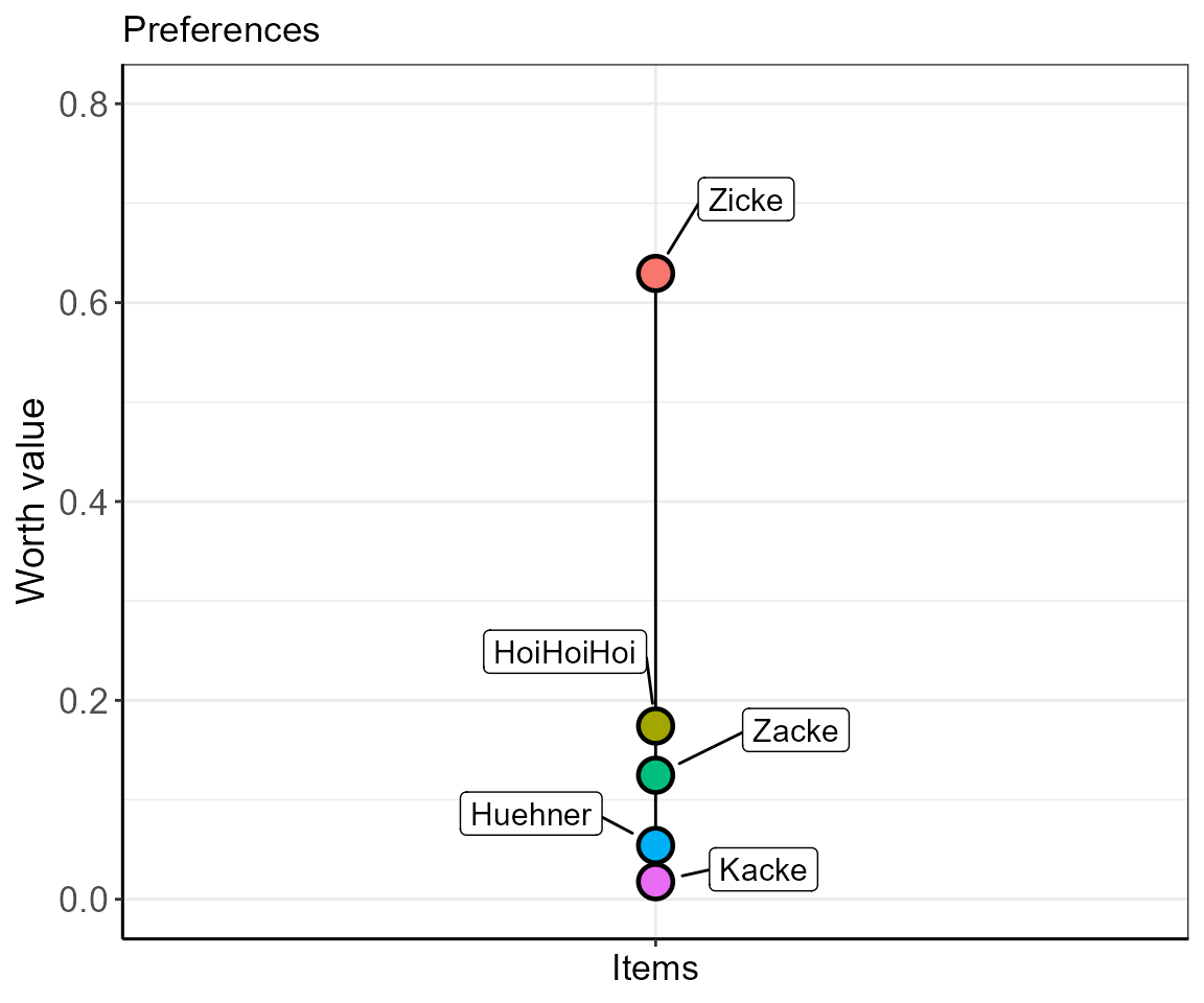

In this plot, you see that the item “HoiHoiHoi” ranks between “Zicke” and “Zacke” scaling closer to “Zacke”. However, this plot conceals the fact that the data for “HoiHoiHoi” are incomplete, and thus the ranking shown is also only limited in its validity. In order to cope for such uncertain data, we introduce the consensus error, i.e., the percentage of disagreement between the individuals that ranked the specific item combinations.

Here, we provide a detailed explanation on how the consensus error is calculated.

In order to calculate and plot the ranking including the consensus error, the function bimeval is used.

The “ZickeZacke” dataset elicits two warnings. The warnings indicate that the number of subjects tested with the “HoiHoiHoi” item may be too low (“HoiHoiHoi” was only rated by 3 of the 4 subjects while all other items were rated by all 4 subjects).

The second warning shows that the number of other items tested against the “HoiHoiHoi”-item may be too low. To get more reliable results, both values should be increased. For the sake of our example, we continue with the incomplete set of data.

w_errors   <- bimeval(ydata     = predat, 
                      worth     = worth$worth, 
                      GT        = GT, 
                      simOpt    = simOpt,
                      showPlot  = TRUE,
                      ylim      = c(0,0.8))
#> Warning in bimeval(ydata = predat, worth = worth$worth, GT = GT, simOpt = simOpt, : simsalRbim: No. of SUBJECTS WARNING!
#>                 The number of subjects you have provided for testing the
#>                 simOpt='HoiHoiHoi' item is probably insufficient!
#>                 Try increasing the number of subjects.
#>                 You are currently below 80% data coverage for
#>                 that item.
#>                 The consensus error may be biased!
#>                 Your provided-to-simulated subjects ratio is at: 75%.
#> Warning in bimeval(ydata = predat, worth = worth$worth, GT = GT, simOpt = simOpt, : simsalRbim: No. of ITEMS WARNING!
#>                 The number of item tests you have provided for testing the
#>                 simOpt='HoiHoiHoi' item is probably insufficient!
#>                 Try increasing the number of item combinations.
#>                 You are currently below 80% item coverage for
#>                 that item.
#>                 The consensus error may be biased!
#>                 Your provided-to-simulated items ratio is at: 50%.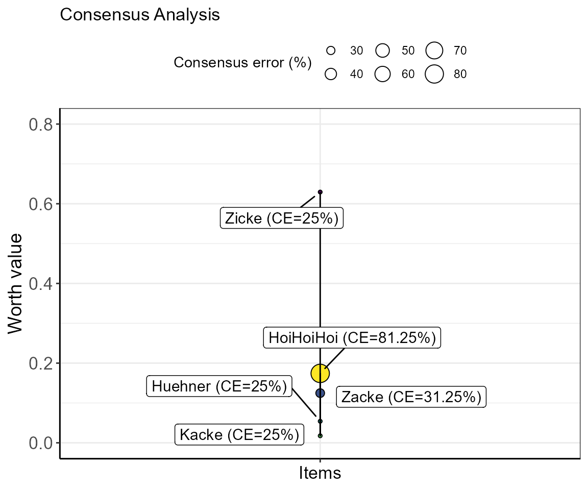

The size of the bubble indicates the consensus error of each item. This means, the smaller the bubble (or error) the more agreement there is between subjects regarding the positioning of the respective item. In the example of the item “Zicke”, the value of 25% indicates that all subjects that were presented with item combinations including “Zicke” showed 25% disagreement. The position of “Zicke” can, therefore, not be warranted.

In contrast, the consensus error for item “HoiHoiHoi” was calculated with 81.25%. Meaning that ~81% of subjects indicated different preferences in item combinations including “HoiHoiHoi”. Conversely, also the consensus errors for “Zacke” and “Kacke” are >0 owing to the fact that in these data the subjects did not agree on whether “HoiHoiHoi” was rated higher or lower than these items. Taken this together with the displayed warnings (only 3 of 4 subjects rated “HoiHoiHoi” and “HoiHoiHoi” was only compared to 3 of the 4 other items) for that item, the positioning of it is relatively insecure.

Example 2 - uninformed item position simulation

Once the rank and scale of a number of items is known (i.e., the ground truth data), one might want to sequentially extend it with additional items. For extending an existing scale it might not be feasible to conduct all possible binary preference tests. In cases of incomplete binary comparisons, we propose a simulation approach, allowing to rank items with a reasonable precision.

Not tested item combinations are attributed a tie. In the GNM model, results can assume the states c(-1,0,1) [=c(worse, equal, better)]. By randomizing this outcome, the degrees of freedom for the unknown combinations get constrained so that the estimate of the item becomes more secure. This logic is used in the bimUninformed function to simulate an uninformed worth calculation for optimal item positioning.

We differentiate between ‘uninformed’ (this example) and ‘informed’ (see example 3) item positioning simulations. In uninformed item positioning, no a priori knowledge about item transitivity (e.g., if A<B and BC, the triplet is considered as being intransitive) is available. Hence, in uniformed simulations, transitive as well as intransitive item combinations derived from the randomization are included. In the informed version of the simulation, a percentage (e.g., tcut=70) for the maximum number of accepted intransitivity can be set.

The function bimUninformed allows the determination of the number of necessary randomization steps. Here, for any number of randomization steps, an ANOVA with a correction for multiple comparisons (MCP) is used to compare the worth values within a simulation run. As long as the calculated worth values are not significantly different, the items’ position is not secured.

Each increase in the number of randomizations will decrease the number of degrees of freedom. Eventually, this will lead to a saturation of the mean adjusted p-values in the MCP tests and a decrease in errors. We define the number of required randomizations as the point at which the adjusted p-value hits zero. For ambiguous data, this can mean a lot of required randomizations. This is a heuristic! So, be prepared to try this out manually for your data.

# We will run 100 randomizations in this example to find the optimal cutoff
cutoff     <- bimUninformed(ydata      = predat, 
                            GT         = GT,
                            simOpt     = simOpt, 
                            limitToRun = 50, 
                            ylim       = c(-0.7,1.2) )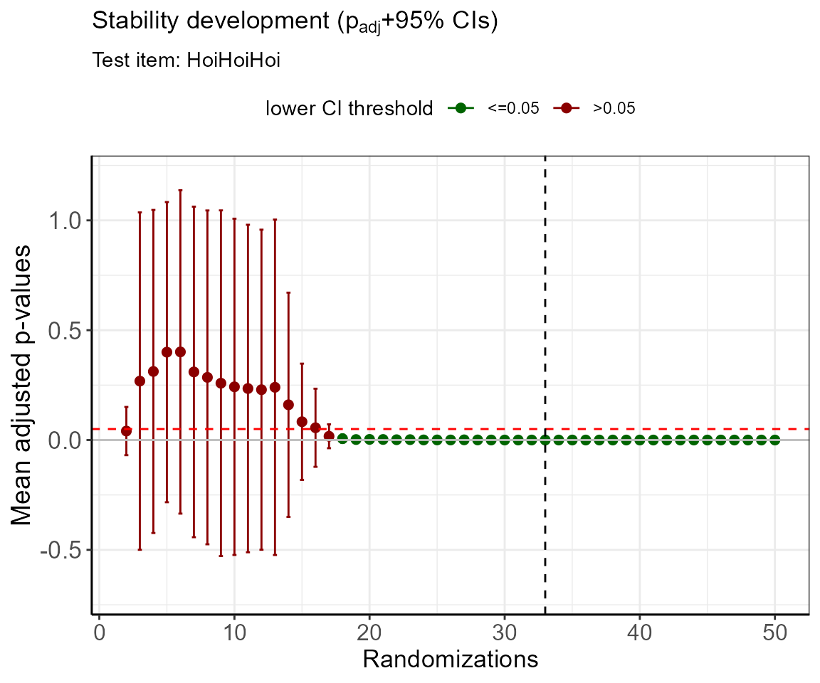

cutoff$cutoff
#> [1] 33

Note: The simulation of adjusted p-values can include confidence intervals that exceed 1 and fall below 0, especially in the beginning of the randomization process. This is owed to the fact that in these cases, the model is statistically underpowered. After determining the cutoff value, the adjusted p-value +- confidence interval should be 0.

The simulation proposes 33 randomization runs in order to reach a sufficient distinction between the items. This result can be displayed with 95% confidence intervals using the bimpos function. Here, we will insert the number of required randomizations.

pos        <- bimpos(ydata      = predat, 
                     GT         = GT, 
                     simOpt     = simOpt, 
                     limitToRun = cutoff$cutoff, # 65
                     showPlot   = TRUE )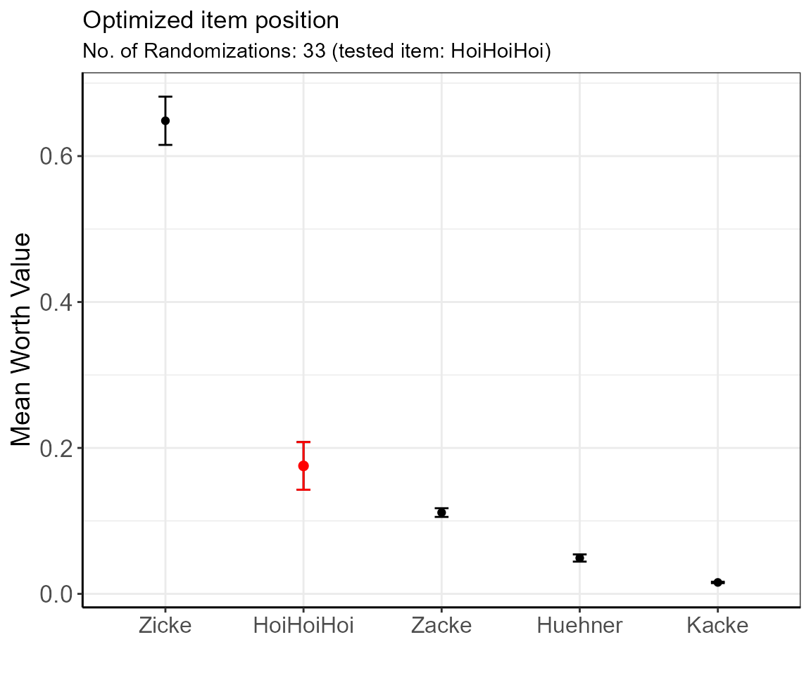

item	Mean.W	SD.W	n.W	se.W	lower.ci.W	upper.ci.W	pos
Zicke	0.6483987	0.0932934	33	0.0162403	0.6153183	0.6814791	1
HoiHoiHoi	0.1753928	0.0920534	33	0.0160244	0.1427521	0.2080335	2
Zacke	0.1114066	0.0168024	33	0.0029249	0.1054487	0.1173645	3
Huehner	0.0491281	0.0139419	33	0.0024270	0.0441845	0.0540716	4
Kacke	0.0156739	0.0027293	33	0.0004751	0.0147061	0.0166417	5

The table shows the ordered estimated mean worth values for each item with errors. In the presented example, the items’ positions are secured as there are no overlapping 95% confidence intervals.

Here, and in comparison to the results in example 1 (low confidence in the position of “HoiHoiHoi”), we can be rather confident that “HoiHoiHoi” is in position 2 (if in doubt, increase the number of randomizations for more precision until the items are separated).

Example 3 - informed item position simulation

In the last example, we will perform an informed simulation of the data, including incomplete binary comparisons. In an informed simulation, transitive choices and a defined maximum of intransitive choices are considered. The user can opt between two evaluation metrics and/or can make an informed decision based on both. With the filter.crit object, either the consensus error (“CE”) or the standardized transitivity ratio (“1-Iratio”) is shown. This way, we can estimate which choices were inconsistent and include this in our evaluation. We use a frequency distribution to decide on the most likely position of the simulated item.

Example Simulation using the Consensus Error (CE)

frqnc      <- bimsim(rawdat      = dat, 
                     GT          = GT, 
                     simOpt      = simOpt,
                     filter.crit = "CE",
                     limitToRun  = 50, 
                     tcut        = 0.85,
                     ylim        = c(0,0.45))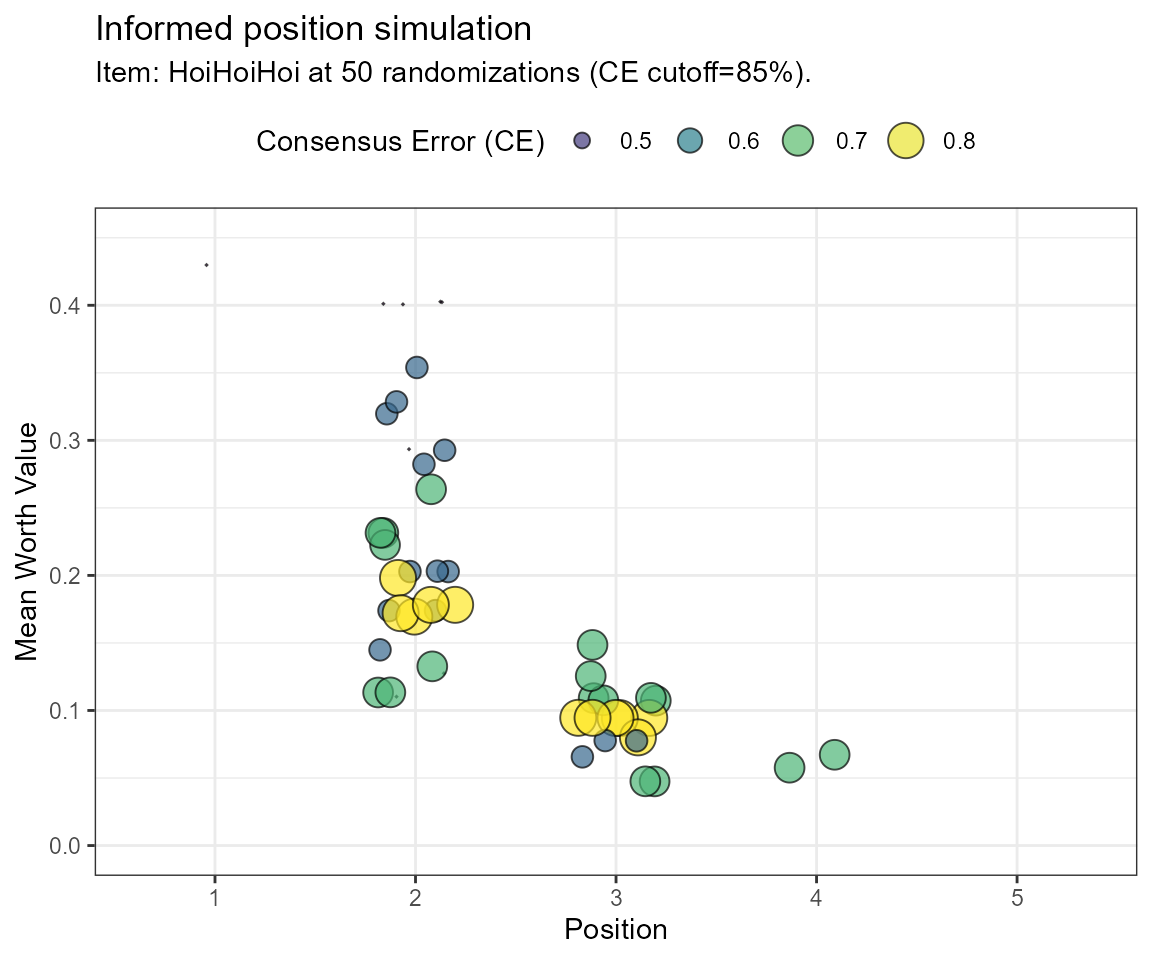

Position	Frequency
1	0.02
2	0.60
3	0.34
4	0.04

Example Simulation using the intransitivity ratio (Iratio)

# Note: the calculation if Iratios takes longer!
frqnc      <- bimsim(rawdat      = dat, 
                     GT          = GT, 
                     simOpt      = simOpt,
                     filter.crit = "Iratio",
                     limitToRun  = 65, 
                     tcut        = 0.80,
                     ylim        = c(0,0.45))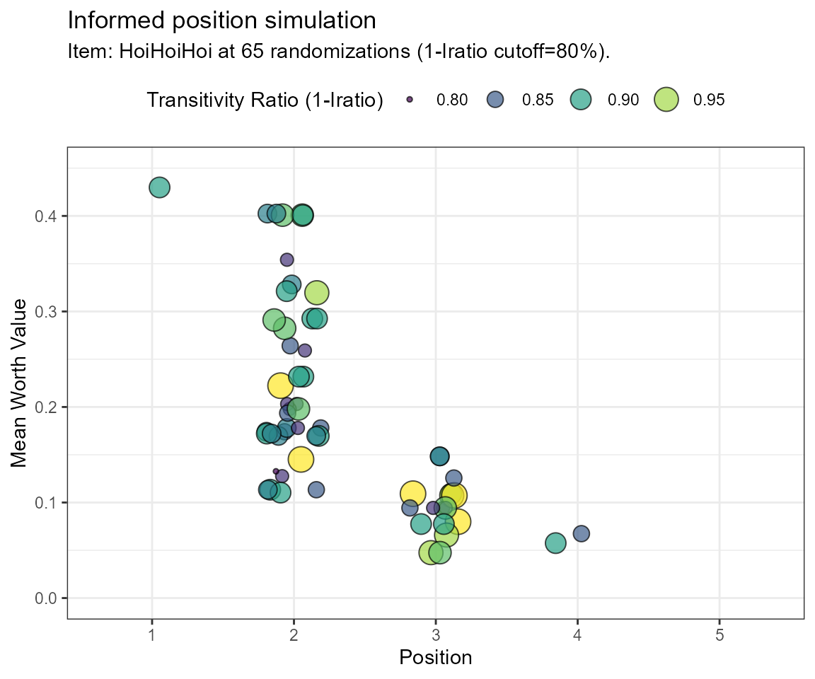

Position	Frequency
1	0.0163934
2	0.6557377
3	0.2950820
4	0.0327869

Note, that even though the calculations are different in both approaches, the final distributions are equal in this case. Position 2 shows the most frequent occurences for the simOpt item and may, therefore, be a reasonably well-placed position estimate.

References

1. Hatzinger R, Dittrich R: prefmod: An R Package for Modeling Preferences Based on Paired Comparisons, Rankings, or Ratings. Journal of Statistical Software 2012, 48:1–31.

Steven R. Talbot

Dana Pfefferle

Ralf Brockhausen