tiefightR Vignette
Steven R. Talbot
2020-07-14
Source:vignettes/tiefightR_Vignette.Rmd
tiefightR_Vignette.RmdtiefighR for preference testing
Preference tests are a valuable tool to measure the “wants” of individuals and have been proven to be a valid method to rate different commodities. The number of commodities presented at the same time is, however, limited and in classical test settings usually, only two options are presented. In our paper, we evaluate the option of combining multiple binary choices to rank preferences among a larger number of commodities. The tiefightR package offers the necessary tools to test selections of commodities and to obtain an estimate of their relative position.
Dependencies
tiefightR uses the following packages as dependencies (in no particular order). Installing tiefightR will usually take care of this. However, sometimes single dependencies can cause problems and have to be installed manually.
“magrittr”(Bache and Wickham 2014),
“tibble”(Müller and Wickham 2020),
“dplyr”(Wickham et al. 2020),
“reshape2”(Wickham 2007),
“prefmod”(Hatzinger and Dittrich 2012),
“gnm”(Turner and Firth 2020),
“ggplot2”(Wickham 2016),
“ggpubr”(Kassambara 2020),
“foreach”(Microsoft and Weston 2020),
“viridis”(Garnier 2018),
“Rmisc”(Hope and Hope 2016)
“doRNG”(Gaujoux 2020)
“ggsci”(Xiao 2018)
The following function can be used to install single packages - or just the missing ones from CRAN.
install.packages("paste missing package name here ")
General concept of the tiefightR package
For data binarization, a preference threshold for the ties is needed (by default this is 50% for an equal commodity selection Likelihood). In the case of ties, the binary response variable is randomized. Therefore, the analysis has to be repeated multiple times for getting more robust estimates of the tested commodities’ position in the data.
Further, the tiefighteR package offers simulation capabilities. This will help to determine the position of individual items without having to test the whole data set. The simulation will randomly test an item against all remaining combinations. These calculations are combined with an estimate on the intransitivity which acts as a quality sign for the found position. The simulation results can indicate similar data and how new commodities can be positioned.
Data
We conducted experiments with rhesus macaques, mice, and humans to validate the ranking method across species. These data sets are included in the package and are called human, mouse, and rhesus. The response variable for humans is binary and for rhesus and mouse it is continuous (i.e., the amount of drank liquid). To harmonize the analysis, continuous data will have to be binarized.
The following example (mouse) shows how the raw (input) data need to be structured. The “pref_img1” is the binary response variable.
head(tiefightR::mouse)
#>         date animalID  side fluidType numOF_visits_with_Licks
#> 1 09.07.2018  ro_ge_4  left       HCl                       7
#> 2 09.07.2018  ro_ge_4 right      NaCl                      17
#> 3 10.07.2018  ro_ge_4  left      NaCl                       1
#> 4 10.07.2018  ro_ge_4 right       HCl                      22
#> 5 09.07.2018  ro_si_4  left       HCl                      13
#> 6 09.07.2018  ro_si_4 right      NaCl                      21
#>   total_visits_withLicks combinationWith test_no no_licks total_licks
#> 1                     21            NaCl       1      543        1740
#> 2                     21             HCl       1     1197        1740
#> 3                     23             HCl       1        1        1528
#> 4                     23            NaCl       1     1527        1528
#> 5                     34            NaCl       1      722        2097
#> 6                     34             HCl       1     1375        2097
The column names in different data sets can be different. Therefore, the functions have fields that need specification. The following names should be adjusted when they are different (e.g. in the tie_worth function).
 RF        = "fluidType"                # name of the reference fluid variable (default = "img1")
 CF        = "combinationWith"          # name of the combination fluid variable (default = "img2")
 id        = "animalID"                 # subject IDs (default = "ID")
 RV        = "numOF_visits_with_Licks"  # name of the response variable (default = "pref_img1")
How many tests are required?
The output of the tie_worth function is worth values that can be ranked for the position. When ties are present (or introduced), the worth values will shift. The question is: when can a user be certain that a position is legit when ties are present? To stabilize the position in terms of worth values, we use the power of the central tendency shift of the mean. The more often a random test is repeated, the more stable the mean becomes. To generalize the different distances we calculate the (Euclidean) distance matrix of the worth values at each randomization step and report the average distance over the number of randomizations. It can be expected that the mean Euclidean distance and the corresponding variance stabilize.
Consider the following worth plot for binary mouse data. The distance between two data points is simply the difference between worth values. In the distance matrix, the distances for all combinations are calculated.
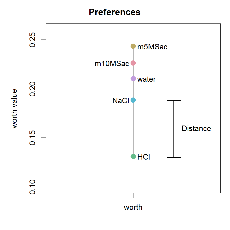
Of course, this only works when ties are present! Otherwise, there would be nothing to randomize.
How to determine an opitmal cutoff?
The largest change in Euclidean distance occurs within the first randomization steps. The corresponding uncertainty of the distances corroborates this (95% CIs). The package contains two specific functions (tie_cicheck and tie_cutoff) that can be used for thresholding. The tiefightR_cutoffs Vignette shows an example of how a reasonable cutoff for a discrete number of randomizations can be achieved for a specific set of data.
Testing single commodities
With this knowledge, individual items from the commodity list can be tested. The tie_test function was specifically designed to test individual combinations. For example, if the position of the NaCl item is to be tested (e.g., at 50 randomizations), the user combines this with any other item combination from the list. As a further criterion (and a sign of good quality), the intransitivity is computed as well. The user can add more items to the tested “against” list for getting more confidence in the positioning of the tested item (hopefully, with lower intransitivity).
#>      against worth pos intrans Ipct   n I_sd  upr   lwr
#> NaCl     HCl  0.19   2   35.33 8.03 440 2.08 40.5 30.16
NaCl is positioned on position 2 (which is the truth, with HCl in position 1). Adding more items can lower the intransitivity (but depends on the individual intransitivities in the data set).
References
Bache, Stefan Milton, and Hadley Wickham. 2014. Magrittr: A Forward-Pipe Operator for R. https://CRAN.R-project.org/package=magrittr.
Garnier, Simon. 2018. Viridis: Default Color Maps from ’Matplotlib’. https://CRAN.R-project.org/package=viridis.
Gaujoux, Renaud. 2020. DoRNG: Generic Reproducible Parallel Backend for ’Foreach’ Loops. https://CRAN.R-project.org/package=doRNG.
Hatzinger, Reinhold, and Regina Dittrich. 2012. “prefmod: An R Package for Modeling Preferences Based on Paired Comparisons, Rankings, or Ratings.” Journal of Statistical Software 48 (10): 1–31. http://www.jstatsoft.org/v48/i10/.
Hope, Author Ryan M, and Maintainer Ryan M Hope. 2016. “Package ‘ Rmisc ’.”
Kassambara, Alboukadel. 2020. Ggpubr: ’Ggplot2’ Based Publication Ready Plots. https://CRAN.R-project.org/package=ggpubr.
Microsoft, and Steve Weston. 2020. Foreach: Provides Foreach Looping Construct. https://CRAN.R-project.org/package=foreach.
Müller, Kirill, and Hadley Wickham. 2020. Tibble: Simple Data Frames. https://CRAN.R-project.org/package=tibble.
Turner, Heather, and David Firth. 2020. Generalized Nonlinear Models in R: An Overview of the Gnm Package. https://cran.r-project.org/package=gnm.
Wickham, Hadley. 2007. “Reshaping Data with the reshape Package.” Journal of Statistical Software 21 (12): 1–20. http://www.jstatsoft.org/v21/i12/.
———. 2016. Ggplot2: Elegant Graphics for Data Analysis. Springer-Verlag New York. https://ggplot2.tidyverse.org.
Wickham, Hadley, Romain François, Lionel Henry, and Kirill Müller. 2020. Dplyr: A Grammar of Data Manipulation. https://CRAN.R-project.org/package=dplyr.
Xiao, Nan. 2018. Ggsci: Scientific Journal and Sci-Fi Themed Color Palettes for ’Ggplot2’. https://CRAN.R-project.org/package=ggsci.